
Data
Machine learning intrusion detection: what the data stages taught us
What we learned building an ML intrusion detector from raw packet capture to live alerts, and which stages were data work.
Computing America. Applications, integrations, data analysis and AI/ML engineering.
Describe the detection
In short
- On our captures, many extreme values were attack traffic, so dropping rows beyond 1.5 times the interquartile range discarded some of it. Switching to clipping at 3 times raised validation F1; the cleaning section gives the size, and why it cannot say which of the two changes mattered.
- Labeling individual packets makes many labels wrong, because a malicious session is full of innocuous traffic. Label flows.
- On our engineered flow statistics, gradient-boosted trees scored F1 0.981 and the convolutional network 0.974, on the same leaked validation split. The gap is too small to rank them.
- Build the pipeline as decoupled, replayable stages, so a crash at stage five doesn't force a re-run of stage one.
- Profile before optimizing the part that feels expensive. In our live detector, inference was sub-millisecond and packet parsing was the slower step.
Four of the seven stages in our intrusion detector are data work, and one cleaning change visibly moved validation F1. We built seven decoupled stages from raw capture to a live detector, with four classical models and a convolutional network at stage five, in roughly fifty hours.
def run_pipeline(self): self.collect_data() # 1. PCAPs -> data/raw_pcaps/{normal,malicious} self.extract_features() # 2. PCAPs -> packet/flow CSVs (scapy) self.clean_data() # 3. dedupe, IQR clip, engineer, scale self.select_features() # 4. ensemble vote across 4 methods self.train_models() # 5. SVM/RF/XGB/MLP + 1D CNN self.evaluate_models() # 6. metrics, ROC, confusion matrices self.deploy_model() # 7. live scapy sniff -> predict_proba -> alertLabel flows, not packets
A naive extractor labels every packet and trains on packets. That yields millions of samples, many with false labels, because a malicious session contains plenty of ordinary handshakes and keepalives. Aggregating packets into flows, keyed on source and destination address, both ports and the protocol, removes many wrong labels, though every flow in a malicious capture still inherits that capture's label. Per flow we compute packet counts, byte totals, duration, packet-size and inter-arrival distributions, and derived rates.
flow_key = ( packet[IP].src, packet[IP].dst, src_port, dst_port, protocol,)flows[flow_key].append(packet)Two flow features, packet rate and average packet size, with one threshold each, already make a detection rule. Move the cuts in the demo below and the confusion matrix moves with them, before any model exists.
Interactive · Applied machine learning
Two features and a threshold rule
drag the sliders
confusion matrix
Clean the data: clip outliers and deduplicate
Switching from dropping rows at one and a half times the interquartile range to clipping at three times it moved validation F1 by roughly 3.5 points. That is one figure for two changes, dropping to clipping and 1.5 to 3 times, so it does not say which one mattered. It is also optimistic: our pipeline oversampled before the train and validation split, so copies of minority rows sat on both sides and inflated the score. Treat 3.5 as the direction of the effect, not a size to expect.
numeric_columns = df.select_dtypes(include=[np.number]).columnsfor col in numeric_columns: if col != 'label': Q1 = df[col].quantile(0.25) Q3 = df[col].quantile(0.75) IQR = Q3 - Q1 lower_bound = Q1 - 3 * IQR upper_bound = Q3 + 3 * IQR df[col] = df[col].clip(lower_bound, upper_bound)Deduplication was the other surprise. Dropping duplicate flows removed about 22% of rows, and we assumed the counter was broken. Scans and floods produce many flows with identical feature vectors, so after a random split the same row sits in both train and test, and a model is partly scored on rows it has already seen. Deduplicate before splitting.
Select features by disagreement
We took an ensemble vote across an F-test, mutual information, recursive feature elimination and random-forest importance, and the value is where they disagree. The F-test measures how far the class means separate, a linear signal. Mutual information, which measures the dependency between two variables (opens in a new tab), counts any relationship with the label, linear or not. Engineered binary features ranked high on mutual information and low on the F-statistic, so selecting with the F-test alone would have dropped real signal.
top_f = set(f_scores['feature'][:20].tolist())top_mi = set(mi_scores['feature'][:20].tolist())top_rfe = set(rfe_features)top_tree = set(tree_features) for feature_set in [top_f, top_mi, top_rfe, top_tree]: for feature in feature_set: feature_counts[feature] = feature_counts.get(feature, 0) + 1 # Keep anything at least two of the four methods asked for.self.selected_features = [f for f, c in feature_counts.items() if c >= 2]Interactive · Feature selection
Feature selection by ensemble vote
mirrors feature_selector.select_best_features()
dot orderF-testMIRFERF imp.
packet_ratepackets_per_secondbyte_rateavg_iatavg_packet_sizestd_iatstd_packet_sizepacket_countdurationtotal_bytesavg_bytes_per_packetmin_packet_sizemax_iatmax_packet_sizemin_iatis_well_known_portis_registered_portdst_portis_dynamic_portsrc_portsyn_ack_ratioprotocoldst_ipsrc_ipfeatures per method (top set)
vote distribution
selected = [f for f, c in counts.items() if c >= 2] does in the project.The convolutional network did not beat boosted trees
The network had the full regularization stack: batch normalization, dropout, weight decay and early stopping. On the same validation split it scored F1 0.974 against 0.981 for gradient-boosted trees, as the output below shows. That split carries the oversampling leak, which favors a model that memorizes rows, so a gap this small may not survive a clean split, and we did not test why. We did not try raw packet sequences, which would be a different pipeline.
validation F1, leaked split
- Gradient-boosted trees0.981
- Convolutional network0.974
The convolutional network scored 0.007 F1 below gradient-boosted trees, on a validation split the oversampling leak inflates: too small a gap to rank them.
SourceStage 6 output of our pipeline, reproduced in this article. Both scores are on the validation split that the oversampling leak inflates, so neither is a clean estimate; a clean split could move both.
The literature points the same way for MLP-like networks. Grinsztajn, Oyallon and Varoquaux benchmarked trees against neural networks on a standardized set of tabular problems and found trees still state of the art. They traced it to three properties: such networks are less robust to uninformative features, are rotation invariant (which discards the meaning of each column), and are biased toward overly smooth solutions, so they struggle with irregular target functions. The benchmark's datasets have heterogeneous columns, as flow statistics do. The finding covers medium-sized data, around ten thousand samples, and says nothing about ten million rows or raw sequences.
Sources
- 1.Why do tree-based models still outperform deep learning on typical tabular data? (opens in a new tab), Grinsztajn, Oyallon & Varoquaux,
- 2.mutual_info_classif (opens in a new tab), scikit-learn
feature F MI RFE Tree votesflow_iat_std * * * * 4fwd_pkt_len_max * * * . 3init_win_bytes_fwd * . * * 3bwd_pkt_len_mean . * . * 2 kept at the threshold--stage 6/7 gradient-boosted trees F1 0.981stage 6/7 1D convolutional net F1 0.974The threshold is a business decision
A classifier doesn't raise alerts. A threshold on its output does, and every position on the slider trades a missed detection against a false one. The math can't say which is right. What does an investigation cost, what does a miss cost, and how many alerts will the receiving team work before closing them unread? Show the receiving team a curve with a handle on it and let them choose.
Interactive · Evaluation
Where to put the alert threshold
mirrors anomaly_detector.alert_threshold
Lower the threshold to catch more attacks (higher recall) at the cost of more false alerts. Raise it for cleaner alerts at the cost of misses. The project ships at 0.7 in config.json, where this synthetic set happens to produce no false positives; around 0.5 both error columns fill and the trade is easier to read.
at this threshold
Three structural decisions that made it survivable
- Every stage writes its output to disk and reads its input from disk, so a crash at stage five doesn't force a re-collection at stage one. Explicit pipeline state records which stages have completed.
- The selected feature column list is written at training time and read back at inference. Column order is part of the contract between training and serving, and rebuilding the list at inference produces confident nonsense with no error.
- One configuration file holds paths, thresholds and hyperparameters, so someone who wasn't there can reproduce a run.
Profile before optimizing
We expected inference to be the live detector's bottleneck, since it feels expensive. Scoring a flow is sub-millisecond. The packet parsing and field extraction in front of it is slower, so throughput means replacing the parser, and touching the model would accomplish nothing.
What we would change next time
- Model the pipeline as a dependency graph, so stages re-run individually, cache by content hash and parallelize.
- Split first and fit the oversampler, scaler, outlier bounds and selector on the training fold only, from day one. We oversampled before the split, and the honest answer to a reviewer asking how leakage was avoided is that it wasn't.
- Version intermediate datasets with the code, so “why did the score drop on Monday” takes two minutes to answer.
- Plot the per-class distribution of every feature before training anything. Half the bugs and most of the wins are visible in those histograms.
Before you commission a model
Write down what you are trying to detect and how you would know you were right. Then hold out a capture from a different day or network, and set how many alerts the receiving team will work before you choose a threshold.
Next step
Tell us what you are trying to detect.
And how you would know you were right. We will say whether the data you already hold can support it, before anybody chooses an algorithm.
- Phone
- (214) 723-2510
- Reply
- A person replies, not a sequence: within one business day, from someone who would be on the engagement.
Packages
Start with a package
Four packages, each with its price on the page. Pick one and buy it online.
$199/month
Billed monthly
$182.42/month
Billed yearly
$499/month
Billed monthly
$457.42/month
Billed yearly
- Scammers stopped from sending email as you
- Your website and systems scanned every week
- Your email settings checked every week
- Everything in the 1 to 10 plan
- Covers up to 50 people
$199/month
after a one-time setup fee
- A site planned, designed and built for you
- Hosting and updates every month
$499/month
Billed monthly
$457.42/month
Billed yearly
$999/month
Billed monthly
$915.75/month
Billed yearly
- Your Google profile, fully set up
- A Google post every week
- 2 social posts a week
- Everything in Get found
- 4 social posts a week
- Your top 10 Google searches tracked
from$500/month
after a one-time setup fee
- Your data gathered from the tools you use
- A first analysis that answers your questions
- New findings every month
Related reading
 AI3 min read
Which AI projects are worth funding: the three conditions
What to check before you fund an applied AI project, and what to build before the model.
 Engineering3 min read
Route optimization: when the shortest path is the wrong objective
How an interactive route planner went from the shortest path to the safest one, and what we learned building it.
 Security5 min read
OT network anomaly detection with fuzzy hashing (TLSH)
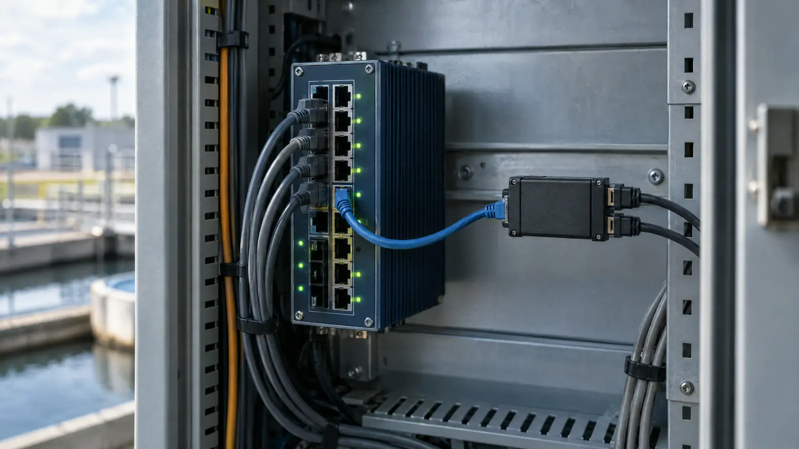
How a TLSH similarity hash over Modbus/TCP packet clusters flags drift, the alternatives that failed, and what the method misses.